If your students have seen that (for a differentiable function on a closed interval) the average rate of change of f always equals the average value of f’, then you are ready to show them a nice way of visualizing the Mean Value Theorem. I think almost every calculus teacher illustrates the MVT with a picture something like this one:
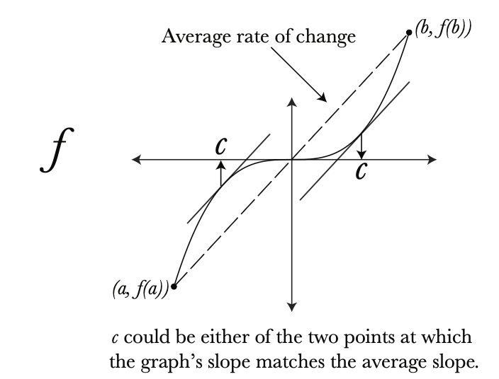
Here, we can see the point(s) at which the average rate of change matches the instantaneous rate of change. If we view the same situation from the perspective of f’, then we get this picture:
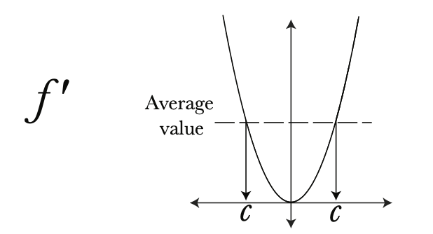
Since the average rate of change of f equals the average value of f’ , the x-values satisfying the MVT for f are precisely the same as those for which the derivative equals its average value.
Phrased in terms of f’, the MVT says this: The function f’ , if it exists everywhere on an interval, must equal its average value somewhere on that interval. And the values of “c” satisfying the theorem are the places where f’ equals its average value.
This way of stating the MVT makes the theorem seem almost obvious: how could a function not ever equal its average value? There is actually a good answer to this rhetorical question: f’ might fail to equal its average value if it has a jump discontinuity. And the point of the MVT is that f’ must fail to exist at any point where it has such a discontinuity. The following example illustrates this:
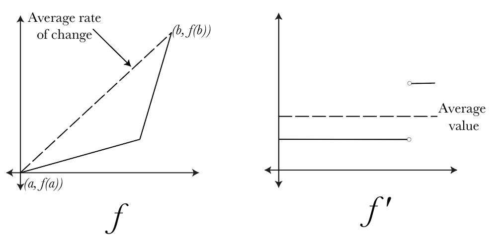
In this case, f’ never equals its average value, because it “jumps over” that average value. And f’ having a jump like this necessarily forces it to be undefined at the point of the jump. This is why the MVT only guarantees that f’ takes on its average value only if f is differentiable everywhere on the given interval.
What happens if we take the example above and “smooth out” the corner on f, making it just rounded enough for f to be differentiable? Then we get something like this:
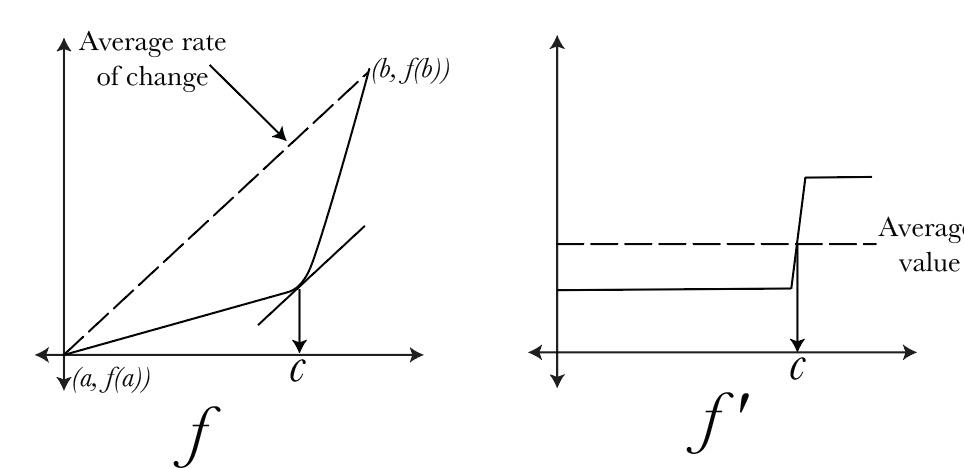
As soon as we “smooth out the corner on f “, the rounded corner means that the slope of f (and thus the value of f’) transitions smoothly from the smaller value to the larger one, and thus takes on all values between its maximum and its minimum.
None of this is a proof of the MVT, but it helps students understand why it feels reasonable, and also why differentiability is a critical part of the theorem.
Looking at the graphs above, an exceptionally astute student will sometimes say something like “wait a minute, can we prove the MVT by applying the IVT to f’ ?” Or “is the MVT basically the integral of the IVT? ” The answer to these questions is “no, sadly it isn’t.” We can’t apply the IVT to f’ because it is possible for f’ to exist and yet not be continuous. The reason that the MVT is such a big deal is precisely that f’ (if it exists on an interval) will always equal its average value, even in situations where it is not continuous. But that’s a story for another post.
If you like this and want a copy of my whole book, please click here
Leave a Reply