Suppose you have done this activity, which has students use a numerical derivative to produce a growth-rate graph based on CDC growth charts. And suppose you have also done this sequence of activities, which introduces students to integration using the energy released by a supernova and culminates in the computation of an accumulation function, showing cumulative energy over time. And perhaps you’ve also had students do this problem, which gets them thinking about the connection between accumulation and rate in the context of COVID. If so, then your students have seen all three pairs of graphs shown below.
If you like this and want a copy of my whole book, please click here
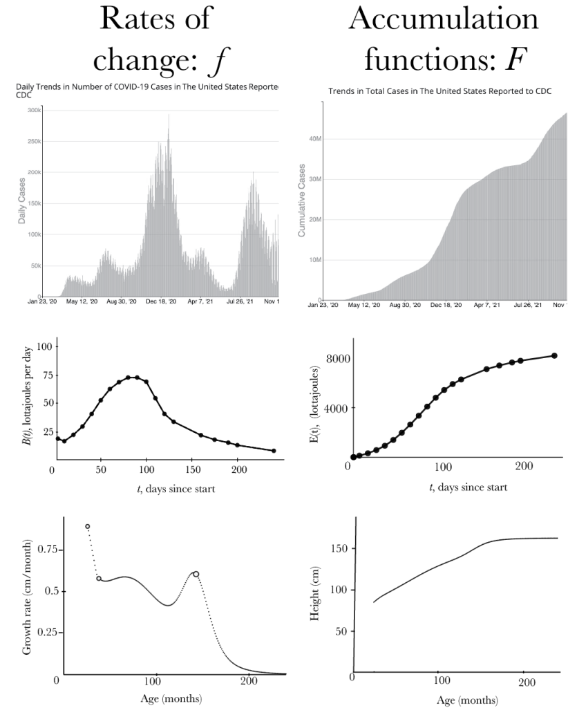
There are many rich conversations to be had about these three pairs. In the growth rate and height graphs (bottom), does the decreasing growth rate after age 12 mean that people shrink? In the COVID graphs (top), how does each of the two graphs show the moment when COVID was most prevalent in the united states? In the supernova graphs (middle pair, showing brightness and cumulative energy), what causes the energy function to flatten out at the end? And why doesn’t the energy function ever decrease?
All of these are excellent conversations to have with students, but the purpose of this post is to consider how these three pairs of graphs relate to the fundamental theorem. The key is this: although these three pairs have different origins, in many ways they have analogous properties. In all three pairs, slope on the right corresponds to a value on the left, and this is true even for the supernova pair, which was produced using an integral. In short, integrating brightness has given us a function (energy) whose derivative is brightness. This is exactly what part 1 of the Fundamental Theorem says: Integrals can be used to construct antiderivatives. Even though the supernova pair was constructed using a Riemann sum (and not a derivative), the effect of this is to produce a derivative-antiderivative pair, brightness and energy.
Similarly, in all three pairs, area on the left corresponds to a change in the value on the right: for example, the area under the growth rate graph gives us the change in height between two times. Critically, this is true even though the height-growth rate pair was constructed using a derivative and not a Riemann sum. Even though an integral wasn’t involved in constructing this pair, it is still true that the antiderivative (height) can be used to evaluate an integral of growth rate. This is part 2 of the fundamental theorem: because growth rate is a derivative of height, it must be true that an area on the growth rate graph is the same as the change in height.
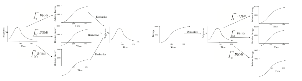
These properties are illustrated in the figure below. Part 1 of the FToC is on the left (integrals produce antiderivatives, i.e. slope on the accumulation function is value on the corresponding rate) and part 2 is on the right (antiderivatives can be used to evaluate integrals, i.e. area on the rate function is change in value on the corresponding accumulation).

Here is an intuitive and holistic view of both parts of the fundamental theorem: a pair of functions f and F has the property that slopes on F correspond to values on f, if and only if they have the property that areas on the graph of f correspond to change in the value of F. The “if” part of this is part 1 of the Fundamental Theorem, the “only if” is part 2.
Another nice visualization of the Fundamental Theorem comes from thinking of part 2 (like part 1) as saying something about an integral-defined function. Specifically, suppose we write part 2 with a variable upper bound \(\scriptsize x_0\) : $$\int_a^{x_0}F^\prime(x){\rm d}x=F(x_0)-F(a).$$ Written this way, part 2 of the FToC clearly makes a claim about the integral of a derivative. If we use “an integral” as a shorthand for “an integral from a fixed lower bound to a variable upper bound,” then part 2 of the fundamental theorem says that an integral of the derivative of F differs from F only by the constant \(\scriptsize -F(a)\). And, of course, part 1 says that the derivative of an integral of f is precisely f.
In short: if we take an integral and then a derivative, we get back where we started, but if we take a derivative and then an integral the result may differ from our original function by the addition of a constant. Viewed this way, the two parts of the FToC really spell out the nature of derivatives and integrals as almost inverse operations: integrals can be inverted by derivatives, but derivatives can only be inverted by integrals up to a difference of a constant, which is why indefinite integrals need a +C.
The two figures below illustrate this perspective on the Fundamental Theorem. Here is part 1, in which different integrals produce different antiderivatives of a given function, all differing by a constant:
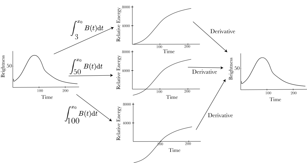
Although different integrals may differ by a constant, the derivative eliminates this constant and returns the brightness function, unchanged from the way it started on the left, regardless of where we start the integral.
Now, here is part 2:
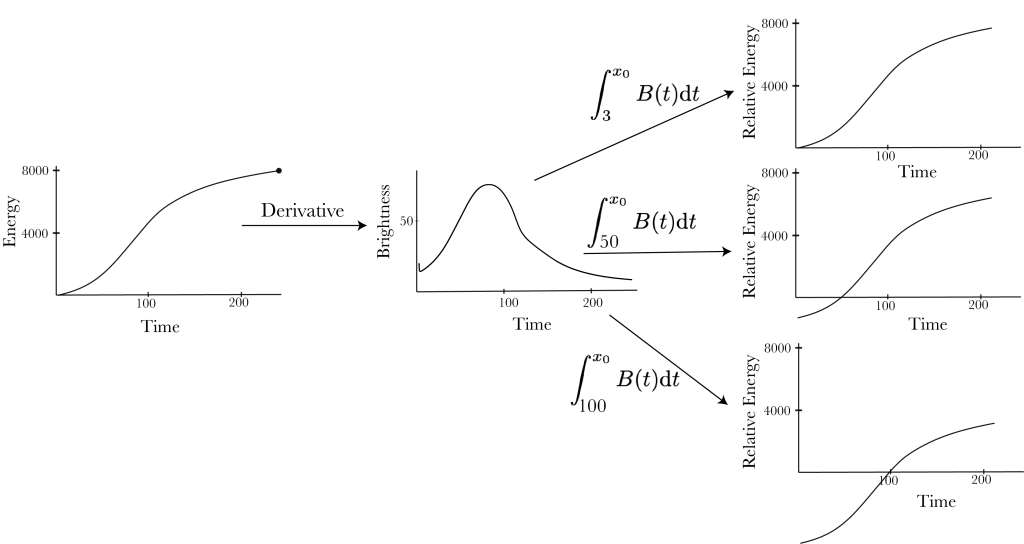
In this case, the integral comes second and so different integrals (which are vertical shifts of each other) give different vertical shifts of the energy graph on the left.
These visualizations may be leveraged as you get into continuous functions. For example, the pair of \(\scriptsize x^2\) and \(\scriptsize 2x\) has all the properties of the pairs above: area on \(\scriptsize 2x\) equals change in value of \(\scriptsize x^2\) and slope on \(\scriptsize x^2\) equals the value of \(\scriptsize 2x\). And (as in the last two figures) integrating \(\scriptsize 2x\) gives a vertical shift of \(\scriptsize x^2\), while differentiating any vertical shift of \(\scriptsize x^2\) results in \(\scriptsize 2x\). Introducing these visuals early can give students a powerful conceptual framework for understanding the Fundamental Theorem and its uses throughout the course.
Up next: tune back in next week for a post with some problems to introduce integration by substitution.